London Cycle-Hire Analytics Platform
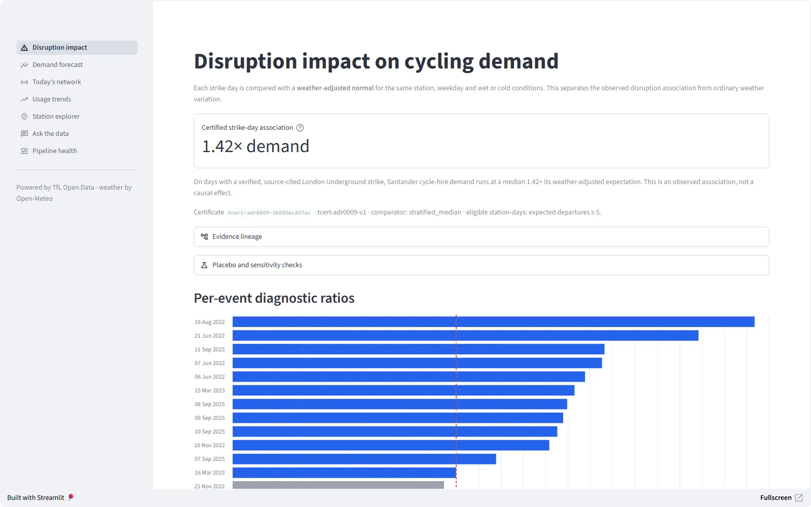
Answers one question well: when London's transport is disrupted, how much extra demand lands on the bikes, and where? A 41.4M-journey PySpark backfill unified across five drifting schema eras, a tested dbt star schema, a LightGBM station-level forecast, and a free always-on live layer refreshed daily by GitHub Actions into committed Parquet — no warehouse to keep alive. Headline: strike days run about 1.4× median demand, up to ~2.3× on the worst full-network strike day.
Key finding
The problem
Transport for London publishes every cycle-hire journey since 2012 — roughly 189M trips across 482 files, with schemas that drift wildly between years. Nobody can answer “what does a tube strike actually do to bike demand, per station?” from the raw archive. This platform unifies it into a clean, tested analytical layer and answers exactly that.
What I built
- A Spark-scale backfill: 41.4M journeys (2022–2026) unified across five distinct file schemas (columns renamed, dropped, and re-ordered between eras), with per-file reconciliation proving no rows are silently lost.
- A tested dimensional model: a dbt star schema (
fact_journey,dim_station,dim_date) with 92 data tests over 17 models, plus a 129-test Python suite, including cross-era station-identity conforming. - Isolating the strike effect: a weather-adjusted baseline separates disruption from weather (disruption days run about 1.42× median demand, 95% CI 1.24–1.61, up to ~2.3× on the worst full-network strike day), so ordinary weather is never mistaken for a strike.
- A learned forecast rather than a median: a LightGBM model predicts station-level daily demand and, by predicting with the disruption flag off, supplies a counterfactual “normal” baseline about 21% more accurate than the median it replaces (held-out 2026, tracked in MLflow).
- A live, durable runtime: a daily GitHub Actions job refreshes line status and dock occupancy into committed Parquet, and the app reads it via DuckDB. No warehouse, no server, nothing to keep paying for.
- Ask it in English: an in-app assistant with keyless exact “quick answers”, plus an optional bring-your-own-key Claude chat over curated, read-only tools.
- Queryable by an agent, not just a person: the warehouse is exposed through a read-only MCP server, so an LLM agent can ask it questions without being handed credentials or write access.
The headline is certified, not just published
The disruption figure is the kind of number that quietly drifts once it is in a README. So it is pinned instead: a certificate SHA-256-hashes the decision record that defines the statistic, the five inputs, the analysis code and the result into a single certificate ID, and verification fails if any of them moves. The statistic string itself — the median station-day ratio of actual to weather-adjusted expected demand — is asserted in code, so relabelling it breaks the build rather than the reader’s understanding.
Getting there needed the inputs to be byte-reproducible, which meant imposing a total order over a dbt-proven unique key and proving three rebuilds identical. Around the headline sit a 95% confidence interval from a cluster bootstrap over event days (1.24–1.61 across 13 events), a day-of-week-matched placebo returning a null median of 1.00 at p < 0.001, and a sensitivity battery over nine weather thresholds. The claim is classed as an observed association, and never as causation.
The Spark ↔ Python boundary
The right tool for each job, documented as an ADR: Spark for the multi-era historical backfill where schema drift and volume justify it; plain Python for the kilobyte-sized daily API pulls where Spark would be theatre. Knowing when not to use the big tool is the point.
Honest limits
TfL publishes journey data in bulk with a ~1–2 month lag, so the workflow deliberately separates historical quantification from live monitoring — it never claims real-time trip prediction (recorded as an ADR). The live demo runs on Streamlit’s free tier and can take ~30s to wake.